At least once a week, and often more frequently, many New Zealanders work their neighbourhood trapping lines. This involves visiting a series of traps set for rodents, hedgehogs, mustelids, or possums to see if there are any new kills. They do this as a community service, helping to rid New Zealand of introduced mammalian predators that are destroying native fauna and flora. Their efforts are now encompassed by an extraordinary government funded initiative called Predator Free New Zealand 2050 (see also “Improving the world for birds” and references within).
An important question is how effective are these neighbourhood trapping efforts? Although many neighbourhood groups contribute citizen science data to databases such as Trap.NZ and CatchIT, there seem to be relatively few scientific analyses of the citizen science datasets. In this article, I examine data from a neighbourhood trapping group at Huia which is surrounded by the Waitakere Ranges Regional Park to the west of Auckland, New Zealand. There are a number of trapping efforts in the Waitakeres (see Predator Free Waitakere Ranges Alliance). Our neighbourhood effort, the Huia Trapping group, was started four years ago, providing data on over 1,100 predator catches at the time of writing.
Neighbourhood trapping effort
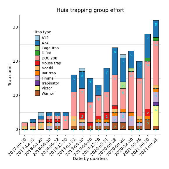
In this contribution, I first examine how our neighbourhood trapping has evolved in terms of the numbers of traps deployed and the types of traps set. Neighbourhood trapping effort at Huia has greatly increased in the past four years (Figure 1). Effort increased from two to five traps deployed in any given quarter of 2018 to over 30 traps deployed in 2021. The diversity of traps used also increased over time. Our most commonly used traps are the conventional DOC200 and automated A24 traps which target rats, mice, and hedgehogs. This year we added D-traps and Victor traps for rats and mice. We also have Timms, Warrior and Trapinator traps targeting possums.
Effectiveness of neighbourhood trapping
With increasing effort, it is important to incorporate the number of traps deployed into any analysis of catch rates. We also need to stratify the data by trap type, target animals, and trap location. This is because differences between trap types, animal behaviour, and the habitats on different neighbours properties could bias the results of analyses. We lack data on how many times traps are sprung without a catch, how frequently traps are checked and found empty, or how often predators approach but do not engage with traps.
These limitations make it impossible to calculate trap efficiencies or encounter probabilities from the citizen science data. While other controlled studies address these questions, an advantage of some citizen science trapping data is that they span longer time periods.
I examined the temporal trends in catches by trap type to determine if catch rates have changed over time. In this analysis, I assume that changes in catch rates reflect changes in target animal local densities. If catch rates are initially high and then decline steeply, we can infer that trapping is knocking down the abundance of predators in the neighbourhood.
By calculating catch rates we can determine whether our neighbourhood trapping effort is having an effect. Catch rates of rats and mice by our two commonest trap types, the DOC200s and A24s, peaked in the first active year for trapping (Figure 2). After 2018, catch rates declined and fluctuated around much lower values (Figure 2). This suggests that trapping knocked down the numbers of rats and mice in the first year (Figure 2), and subsequently numbers remained suppressed as our trapping effort increased (Figure 1). We can also see that initial catch rates by A24 traps were almost an order of magnitude higher for rats than for mice (Figure 2A & C). DOC200 catch rates for rats were initially about four times greater than for mice (Figure 2B & D).
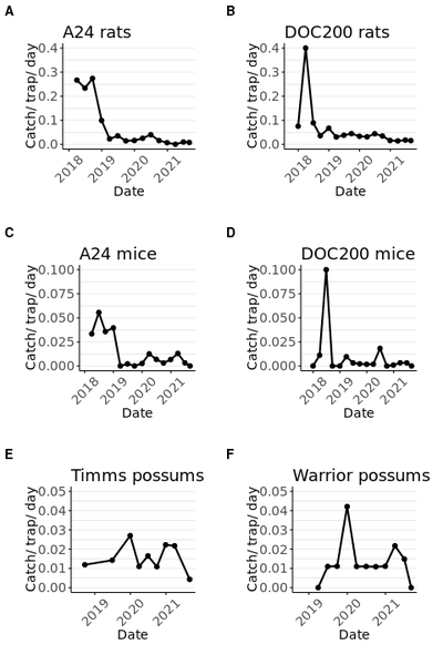
We did not observe the same knockdown effect for possums (Figure 2E & F). Possum catch rates were lower than for either rats or mice, and also did not show a peak in the first year of trap deployment. This may be related to the territorial nature of possums. Males range more widely than females, and it can take as long as 8 weeks or more for possums to reoccupy a habitat where previous occupants have been trapped.
Comparing catch rates of conventional and automated traps
New technology has the potential to reduce the labour of checking traps and changing lures. Our two most commonly used trap types are the conventional DOC200 boxed snap trap and the Goodnature A24 automated trap. In a neighbourhood environment where traps are checked as frequently as a couple of times a week, are the catch rates of automated traps higher than conventional traps like the DOC200? Alternatively, is there any evidence that the automated traps are less effective than the more conventional traps?
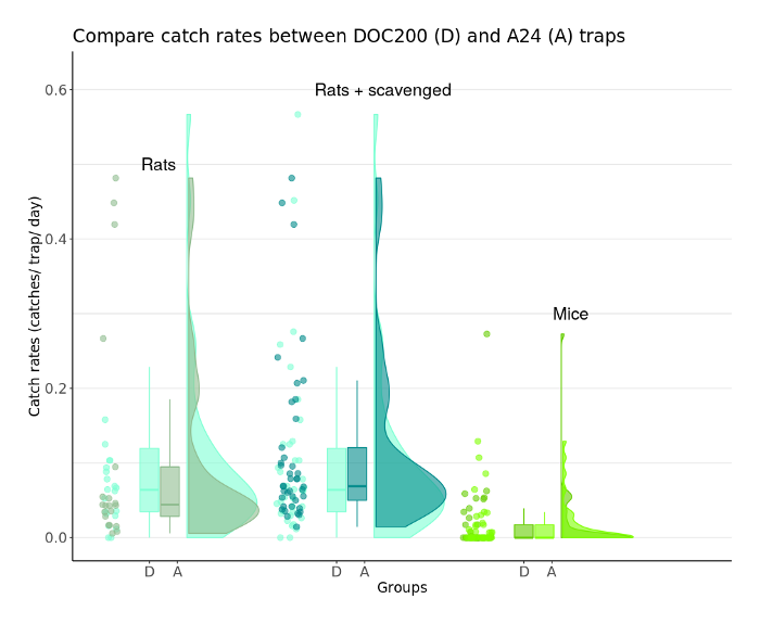
I compared the catch rates of the DOC200 and A24 traps using a simple exploratory data analysis. Figure 3 shows a scatterplot, boxplot and distribution of the catch rates for each trap type, separating the rat and mouse catches. Data are from a single neighbours property to reduce spatial variability. Scavenged catches record a strike by the automated A24 trap when no carcass was found. This usually means the catch was removed by a cat or a rat before the trap was checked.
The catch rates for the two trap types are very similar (Figure 3). The data for both trap types are highly skewed because catch rates are much higher in some months. This is more noticeable for rats than mice. Median values (horizontal lines in the box plots) are very close for the both trap types, and the inter-quartile ranges (the boxes) for both DOC200 and A24 traps overlap. We found no evidence that the automated A24 traps were either more or less effective than the conventional DOC200 traps. These findings suggest that the benefit of the automated trap may derive mainly from the fact that they need to be checked less often, reducing the labour involved.
There may be reluctance to adopt new technology, and suspicion that new methods do not work. The A24 traps are also about three times the cost of the DOC200s. The trade off in checking a trap less often is that kills are more likely to be scavenged by another predator, such as a domestic or feral cat, a stoat, or another rat. The labour saving benefit is offset to some degree by the reduced confidence that catches are real, and not simply an artefact of an inaccurate kill counter. The cost of the traps is also a consideration, especially for neighbourhood trapping where labour is voluntary and so is not costed, whereas the cost of expensive traps is borne by neighbours.
Conclusions
We can answer yes to the question “Does neighbourhood trapping work?”, at least in our neighbourhood at Huia. The answer to the second question posed; “How would we know?” is that analyses of citizen science data in databases like Trap.NZ or CatchIT can provide the evidence.
From this limited analysis of a single trapping group, the evidence indicates that our neighbourhood trapping is having an effect on rat and mice catch rates, and by inference, on rat and mice local densities. This would be difficult to detect without the data provided provided by trappers entering data into a database. An alternative monitoring method is the use of bird song monitors (see my TDS article), but this also requires effort by citizen scientists.
An added benefit of neighbourhood trapping is community engagement for a shared, cooperative goal. We maintain a mail list for updates and information dissemination to all trapping group members. We also have a WhatsApp group for our most active members, where people can ask questions and share their experiences. It’s a great way to get assistance and also helps to maintain motivation. You also get to know your neighbours and strengthen cooperation.
Code
Data were exported from the Trap.NZ site for the Huia trapping group as an ascii file. Using the R tidyverse packages, the data file was imported, character dates converted to class date, variables ordered, selected and renamed, and the subsequent data frame converted to a time tibble.
## import_trapnz_function.R
# Usage:
# source the function
# trapnz <- import.trapnz()# Note: Data were exported from Trap.NZ using menus: Reports/ Trap reports/ Trap records for the full date rangeimport.trapnz <-
function(data.dir = "/mnt/data/dynamic_data/projects/projects2021/trapping/data/",
exported.file = "TrapNZ_export_29_Sept_2021.csv")
{
# load libraries
library(tidyverse)
library(tibbletime)
library(lubridate)
library(readr)
library(tidyr)
# load exported trap.nz data
dat <- paste(data.dir, exported.file, sep = "")
trapnz <- read_csv(dat)
# convert character date to a date object
trapnz <- mutate (trapnz,
Date.new = as.Date(Date, format = "%d %b %Y - %H:%M"))
# order, select and rename variables
trapnz <- arrange(trapnz, Date.new, "Recorded by", Trap)
trapnz <- trapnz %>%
select(Date.new, "Recorded by", Trap, "Trap type", Strikes, "Species caught")
colnames(trapnz) <-
list("date.new", "line", "trap", "traptype", "strikes", "species")
# convert tibble to tibble time
trapnz <- as_tbl_time(trapnz, index = date.new)
# print some summary info
print("########################")
print(paste("Directory: ", data.dir))
print(paste("Exported Trap.NZ file: ", exported.file))
# print(head(trapnz))
# print(tail(trapnz))
trapnz
}
I prepared the data with the following code (prepare_TrapNZ_catch_and_traptype_data.R). After loading libraries, data were loaded using the function above (import_trapnz_function.R), after loading it to the environment using source(). New variables were created from the species character variable, according to tidy data principles. Multiple catches by automated traps, usually where two rats are killed on a single night, were accounted for by multiplying the catch unit category by number of strikes. For successive quarterly (3 month) periods, I summed catches by species, and calculated the number of unique traps for each trap type.
## prepare_TrapNZ_catch_and_traptype_data.R# load libraries #################
library(tidyverse)
library(tibbletime)
library(lubridate)
library(readr)
library(tidyr)# load data ###########
### load, sort, subset trap.nz data
source(
"/mnt/data/dynamic_data/projects/projects2021/trapping/r/import_trapnz_function.R"
)
trapnz <- import.trapnz()# create new variables for catches by species ################
series2 <- trapnz
series2 <- mutate (
series2,
# Date.new = as.Date(Date, format = "%d %b %Y - %H:%M"),
rat_catch = ifelse (series2$species %in% c ("Rat", "Rat - Ship", "Rat - Norway"), 1, NA),
mouse_catch = ifelse (series2$species == "Mouse", 1, 0),
possum_catch = ifelse (series2$species == "Possum", 1, 0),
hedgehog_catch = ifelse (series2$species == "Hedgehog", 1, 0),
stoat_catch = ifelse (series2$species == "Stoat", 1, 0),
scavenged_catch = ifelse (series2$species == "Unspecified", 1, 0)
)
# adjust for multiple catches by A24 traps
series2$rat_catch <- series2$rat_catch * series2$strikes
series2$mouse_catch <- series2$mouse_catch * series2$strikes# quarterly summation of catches by species and number of unique traps
series2 <- arrange(series2, date.new, line, traptype, trap)# group catch data into time bins ########################
quarterly_catches <- collapse_by(series2, "quarter") %>%
dplyr::group_by(date.new, traptype) %>%
dplyr::summarise_if(is.numeric, sum, na.rm = TRUE)
quarterly_catches <- arrange(quarterly_catches, date.new, traptype)# group numbers of individual traps into time bins
quarterly_traptype <- collapse_by(series2, "quarter") %>%
dplyr::group_by(date.new, traptype) %>%
dplyr::summarise(trap_count = length(unique(trap)))
quarterly_traptype <- arrange(quarterly_traptype, date.new)# save the data ####################
Huia_results = list(quarterly_catches, quarterly_traptype)
save(Huia_results, file = "/mnt/data/dynamic_data/projects/projects2021/trapping/data/tidy_catch_traptype_TrapNZ.dat")
The data were used to create Figure 1 using the code below (trapping_effort_over_time_stacked_barplot.R). After loading libraries, I used a couple of theme options to improve the plot. Data saved by the code above (prepare_TrapNZ_catch_and_traptype_data.R) were loaded. I then plotted a stacked barplot using ggplot with a manually specified colour palette for categorical data, tweaking the display to show angled x-axis labels, and to show the counts for numbers of traps in each of the stacked bar segments.
### trapping_effort_over_time_stacked_barplot.R# libraries #######
library(tidyverse)
library(tibbletime)
library(lubridate)
library(gridExtra)
library(ggpubr)
library(RColorBrewer)
library(colorspace)
# custom theme settings ##########
theme_smcc <- function() {
# theme_bw() +
theme(
text = element_text(family = "Helvetica Light"),
axis.text = element_text(size = 14),
axis.title = element_text(size = 14),
axis.line.x = element_line(color = "black"),
axis.line.y = element_line(color = "black"),
panel.border = element_blank(),
panel.grid.major.x = element_blank(),
panel.grid.minor.x = element_blank(),
panel.grid.minor.y = element_line(colour = "grey80"),
plot.margin = unit(c(1, 1, 1, 1), units = , "cm"),
plot.title = element_text(
size = 18,
vjust = 1,
hjust = 0.5
),
legend.text = element_text(size = 12),
legend.position = c(0.2, 0.6),
legend.key = element_blank(),
legend.background = element_rect(
color = "black",
fill = "transparent",
size = 2,
linetype = "blank"
)
)
}theme_angle_xaxis <- function() {
theme(axis.text.x = element_text(
angle = 45,
hjust = 1,
vjust = 0.95
))
}# load data ###################
load(file = "/mnt/data/dynamic_data/projects/projects2021/trapping/data/tidy_catch_traptype_TrapNZ.dat")quarterly_trap_type <- as.data.frame(Huia_results[2])
quarterly_trap_type <- arrange(traps, date.new, trap_count)# plot ###############
png(
"/mnt/data/dynamic_data/projects/projects2021/trapping/figures/trapping_effort_over_time_stacked_barplot.png",
width = 580,
height = 580
)quarterly_trap_type$date_char <-
as.character(quarterly_trap_type$date.new) # to allow bar width adjustmentmypalette <- brewer.pal(12, "Paired")
legend_title = "Trap type"trapping_effort_over_time_stacked_barplot <-
ggbarplot(
data = quarterly_trap_type,
x = "date_char",
xlab = "Date by quarters",
y = "trap_count",
ylab = "Trap count",
label = TRUE,
lab.pos = "in",
lab.col = "cyan1",
fill = "traptype",
title = "Huia trapping group effort"
) +
scale_fill_manual(legend_title, values = mypalette) +
theme_smcc() +
# x-axis adjustment
theme_angle_xaxis()# save the plot
print(trapping_effort_over_time_stacked_barplot)
dev.off()
The time series of catch rates by trap type and species in Figure 2 were created as follows. Data saved by the code above (prepare_TrapNZ_catch_and_traptype_data.R) were loaded. I’ve folded the code segments for loading libraries and the previously shown custom theme to save space. Quarterly catches and trap counts were filtered by trap type before calculating catch rates as catches/ trap/ day. Six individual plots were then created before assembling them into a panel plot.
## explore_multiple_catches.R# load libraries #######
...# custom theme settings #############
...# load data ###################
load(file = "/mnt/data/dynamic_data/projects/projects2021/trapping/data/tidy_catch_traptype_TrapNZ.dat")catches <- as.data.frame(Huia_results[1])
catches <- arrange(catches, date.new, traptype)traps <- as.data.frame(Huia_results[2])
traps <- arrange(traps, date.new, trap_count)# traps ######################
# filter by trap type
# A24
catches_a24 <- filter(catches, traptype == "A24")
traps_a24 <- filter(traps, traptype == "A24")catches_and_traps_a24 <-
select(catches_a24, c(date.new, traptype, rat_catch, mouse_catch))interval <- c(NA, diff(catches_and_traps_a24$date.new))catches_and_traps_a24 <- mutate(
catches_and_traps_a24,
trap_count = traps_a24$trap_count,
.after = traptype,
rat_catch_rate = rat_catch / trap_count / interval,
mouse_catch_rate = mouse_catch / trap_count / interval
)
head(catches_and_traps_a24)# DOC200
catches_doc200 <- filter(catches, traptype == "DOC 200")
traps_doc200 <- filter(traps, traptype == "DOC 200")catches_and_traps_doc200 <-
select(catches_doc200, c(date.new, traptype, rat_catch, mouse_catch))interval <- c(NA, diff(catches_and_traps_doc200$date.new))catches_and_traps_doc200 <- mutate(
catches_and_traps_doc200,
trap_count = traps_doc200$trap_count,
.after = traptype,
rat_catch_rate = rat_catch / trap_count / interval,
mouse_catch_rate = mouse_catch / trap_count / interval
)# Mouse trap
catches_mouse_trap <- filter(catches, traptype == "Mouse trap")
traps_mouse_trap <- filter(traps, traptype == "Mouse trap")catches_and_traps_mouse_trap <-
select(catches_mouse_trap, c(date.new, traptype, mouse_catch))interval <- c(NA, diff(catches_and_traps_mouse_trap$date.new))catches_and_traps_mouse_trap <- mutate(
catches_and_traps_mouse_trap,
trap_count = traps_mouse_trap$trap_count,
.after = traptype,
mouse_catch_rate = mouse_catch / trap_count / interval
)# Timms trap
catches_timms_trap <- filter(catches, traptype == "Timms")
traps_timms_trap <- filter(traps, traptype == "Timms")catches_and_traps_timms_trap <-
select(catches_timms_trap, c(date.new, traptype, possum_catch))interval <- c(NA, diff(catches_and_traps_timms_trap$date.new))catches_and_traps_timms_trap <- mutate(
catches_and_traps_timms_trap,
trap_count = traps_timms_trap$trap_count,
.after = traptype,
possum_catch_rate = possum_catch / trap_count / interval
)# Warrior trap
catches_warrior_trap <- filter(catches, traptype == "Warrior")
traps_warrior_trap <- filter(traps, traptype == "Warrior")catches_and_traps_warrior_trap <-
select(catches_warrior_trap, c(date.new, traptype, possum_catch))interval <- c(NA, diff(catches_and_traps_warrior_trap$date.new))catches_and_traps_warrior_trap <-
mutate(
catches_and_traps_warrior_trap,
trap_count = traps_warrior_trap$trap_count,
.after = traptype,
possum_catch_rate = possum_catch / trap_count / interval
)# plots ############################
png(
"/mnt/data/dynamic_data/projects/projects2021/trapping/figures/explore_multiple_catches.png",
width = 480,
height = 720,
)a24_rats <-
ggline(
catches_and_traps_a24,
x = "date.new",
y = "rat_catch_rate",
title = "A24 rats",
size = 1,
# add = "loess",
conf.int = TRUE,
xlab = "Date",
ylab = "Catch/ trap/ day"
) +
theme_smcc() +
theme(axis.text.x = element_text(
angle = 45,
hjust = 0.5,
vjust = 0.5
))
a24_rats <- ggpar(a24_rats, ylim = c(0, 0.4))doc200_rats <-
ggline(
catches_and_traps_doc200,
x = "date.new",
y = "rat_catch_rate",
title = "DOC200 rats",
size = 1,
# add = "loess",
conf.int = TRUE,
xlab = "Date",
ylab = "Catch/ trap/ day"
) +
theme_smcc() +
theme(axis.text.x = element_text(
angle = 45,
hjust = 0.5,
vjust = 0.5
))
doc200_rats <- ggpar(doc200_rats, ylim = c(0, 0.4))a24_mouse <-
ggline(
catches_and_traps_a24,
x = "date.new",
y = "mouse_catch_rate",
title = "A24 mice",
size = 1,
# add = "loess",
conf.int = TRUE,
xlab = "Date",
ylab = "Catch/ trap/ day"
) +
theme_smcc() +
theme(axis.text.x = element_text(
angle = 45,
hjust = 0.5,
vjust = 0.5
))
a24_mouse <- ggpar(a24_mouse, ylim = c(0, 0.1))doc200_mouse <-
ggline(
catches_and_traps_doc200,
x = "date.new",
y = "mouse_catch_rate",
title = "DOC200 mice",
size = 1,
# add = "loess",
conf.int = TRUE,
xlab = "Date",
ylab = "Catch/ trap/ day"
) +
theme_smcc() +
theme(axis.text.x = element_text(
angle = 45,
hjust = 0.5,
vjust = 0.5
))
doc200_mouse <- ggpar(doc200_mouse, ylim = c(0, 0.1))timms_possum <-
ggline(
catches_and_traps_timms_trap,
x = "date.new",
y = "possum_catch_rate",
title = "Timms possums",
size = 1,
# add = "loess",
conf.int = TRUE,
xlab = "Date",
ylab = "Catch/ trap/ day"
) +
theme_smcc() +
theme(axis.text.x = element_text(
angle = 45,
hjust = 0.5,
vjust = 0.5
))
timms_possum <- ggpar(timms_possum, ylim = c(0, 0.05))warrior_possum <-
ggline(
catches_and_traps_warrior_trap,
x = "date.new",
y = "possum_catch_rate",
title = "Warrior possums",
size = 1,
# add = "loess",
conf.int = TRUE,
xlab = "Date",
ylab = "Catch/ trap/ day"
) +
theme_smcc() +
theme(axis.text.x = element_text(
angle = 45,
hjust = 0.5,
vjust = 0.5
))
warrior_possum <- ggpar(warrior_possum, ylim = c(0, 0.05))# panel plot
explore_multiple_catches <-
ggarrange(
a24_rats,
doc200_rats,
a24_mouse,
doc200_mouse,
timms_possum,
warrior_possum,
labels = c("A", "B", "C", "D", "E", "F"),
ncol = 2,
nrow = 3
)print(explore_multiple_catches)
dev.off()
For the last plot, data preparation involved things already covered such as loading the data, subsetting by trap type to select the A24 and DOC200 traps, and grouping the catches by month, instead of by quarter, in this case. The only novel part was creating the array for the raincloud plot.
# # prepare data format for raincloud plot (packing doc200 arrays to match A24 length)
df_plot <- data_2x2(
array_1 = c(gdata_doc200$rat_catch_eff, NA, NA, NA),
array_2 = gdata_a24$rat_catch_eff,
array_3 = c(gdata_doc200$rats_plus_scavenged_catch_eff, NA, NA, NA),
array_4 = gdata_a24$rats_plus_scavenged_catch_eff,
array_5 = c(gdata_doc200$mouse_catch_eff, NA, NA, NA),
array_6 = gdata_a24$mouse_catch_eff,
labels = c("DOC200", "A24"),
jit_distance = 0.075,
jit_seed = 321,
spread_x_ticks = TRUE
)# save the data for raincloud plot
save(df_plot, file = "/mnt/data/dynamic_data/projects/projects2021/trapping/data/tidy_catch_raincloud.dat")
The raincloud in Figure 3 was created using this code using the previously saved data.
## compare_catch_rates_A24_DOC200_by_raincloud.R# load libraries
library(tidyverse)
library(tibbletime)
library(lubridate)
library(gridExtra)
library(ggthemes)
library(ggpubr)
library(ggrepel)
library(readr)
library(raincloudplots)# custom theme settings
...# load saved tidy_catch_raincloud data
load(file = "/mnt/data/dynamic_data/projects/projects2021/trapping/data/tidy_catch_raincloud.dat")# raincloud plots
# colours
col1 = "aquamarine"
col2 = "darkseagreen"
col3 = "darkcyan"
col4 = "chartreuse3"
col5 = "chartreuse"plot_catches <- raincloud_2x3_repmes(
data = df_plot,
colors = (c(col1, col2, col1, col3, col4, col5)),
fills = (c(col1, col2, col1, col3, col4, col5)),
size = 2.5,
# data dot size
# line_alpha = 0, # make lines fully transparent
alpha = 0.6 # transparency
) +
scale_x_continuous(
breaks = c(1.25, 1.4, 2.25, 2.4, 3.25, 3.4),
labels = c("D", "A", "D", "A", "D", "A"),
# labels = c("DOCC200", "A24", "DOCC200", "A24", "DOCC200", "A24"),
limits = c(1, 4.2)
) +
# scale_y_continuous() +
scale_y_continuous(limits = c(0, 0.62)) +
xlab("Groups") +
ylab("Catch rates (catches/ trap/ day)") +
labs(title = "Compare catch rates between DOC200 (D) and A24 (A) traps") +annotate(geom = "text",
label = "Rats",
x = 1.3, y = 0.5,
size = 6) +
annotate(geom = "text",
label = "Rats + scavenged",
x = 2.5, y = 0.6,
size = 6) +
annotate(geom = "text",
label = "Mice",
x = 3.5, y = 0.3,
size = 6) +
theme_smcc()plot_catches
Access for download
Code, data and figures are all available for download using this shared link.